Methodology
Association Rule Mining, or ARM, is a rule-based unsupervised machine learning method for discovering interesting relations between variables in large datasets. It is mostly used on market/transaction data and intended to identify strong rules discovered in databases using Support, Confidence, and Lift rules. The definition and formula for each rule is shown below:
Support measures how frequently the item appears in the dataset, the proportion of transactions in the dataset containing item X. Sup({X}, {Y}) = (numberof X and Y)/Number_of_Transactions
Confidence measures how often the rule is true, which indicates the proportion of the transactions that contain X, which also includes Y. Conf({X}, {Y}) = P ({X}, {Y}) / P({X})
Lift measures the ratio of the observed support to that expected if X and Y were independent. Lift ({X}, {Y}) = Sup({X}, {Y}) / Sup({Y}) * Sup({X})
If the lift is equal, it will imply that the probability of the antecedent and that of the consequent are independent of each other. When two events are independent of each other, no rule can be drawn involving those two events.
If the lift is larger than 1, that lets us know the degree to which those two occurrences are dependent on one another and makes those rules potentially useful for predicting the consequent in future data sets.
If the lift is less than 1, that lets us know the items are a substitute. This means that one item's presence has a negative effect on other items and vice versa.
Maps are an interactive way of showing data that have geo-columns in them. It can offer either a large chunk of geographic locations on earth or a small terrain with great detail.
Dataset
| Dataset | Type | Description | Condition |
|---|---|---|---|
| Transaction Data | Vectorized/Text Data | Derived from Tweets of Hashtag Trump, using code from previous module, this dataset has each row as a tweet associated with the hashtage and each column is a single word | Cleaned |
| County_Female_Percentage.csv | Map Data | Population dataset include FIPS as GEOID and Female Percentage in each county | Cleaned |
| County_Water_Drought.csv | Map Data | Water Drought Area data, includes FIPS as GEOID | Cleaned |
| County_Land.csv | Map Data | County Land Area dataset, includes FIPS as GEOID | Cleaned |
Section A: Prepare Data for Association Rule Mining
This section only uses python for cleaning and preparing transaction data for later activities. The first step is to acqurie tweets from the twitter API. This step also uses code developped from previous module to to do that. After tokenizing each tweets, the words are seperated into a row of words and each row is a tweet.
line_df_1 = pd.DataFrame(temp_line_ls, columns=['Line'])
line_df_raw = line_df_1

line_df_1["Line"].replace('', np.nan, inplace=True)
line_df_1.dropna(subset=["Line"],inplace=True)

from pandas import Series
temp = line_df_1['Line'].str.split(' ').apply(Series, 1)
basket = temp.fillna(' ')
basket = basket.backfill(axis=0)
#basket.dropna(subset=[0],inplace=True)
basket.to_csv("./Transaction.csv")
The raw text file and final csv file are showing below for comparison. The csv file is suitable for ARM and networking tasks/


Section B: ARM in R
This section only uses R for association rule mining tasks. Association rule mining tasks in R are made easy with the library(arules) and library(arulesViz). Apriori function significantly helps ARM tasks include frequent itemsets, association rules, or association hyperedges. The Apriori algorithm also employs a level-wise search for frequent itemsets.
B - 1: Print and Plot Top 10 Support, Confidence and Lift Rules
Printed output from the console window provides direct feedback of rules outcomes.
TweetTrans_rules = arules::apriori(TweetTrans,
                                   parameter = list(support=0.11, conf=1, minlen=2))
Many attempts were made to the parameters of the apriori function. Setting too low will lead to very long computation time; setting too high will yield little results. Ultimately, the apriori functions' parameters are set at sup 0.11, conf 1, and minimum length 2, giving a satisfactory outcome to facilitate findings and general discoveries.
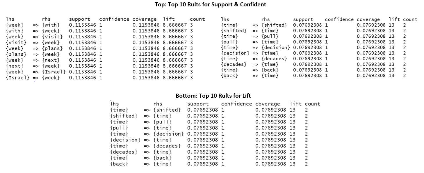
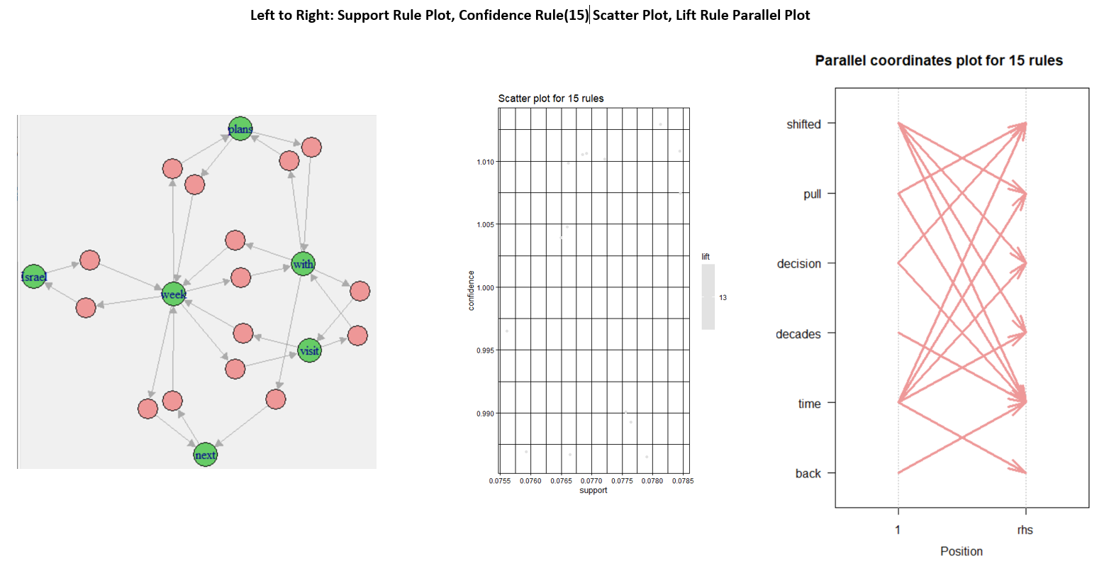
The plotted rules provide the distribution of rules for each rule: Support, Confidence and Lift
B - 2: Additional Visualization
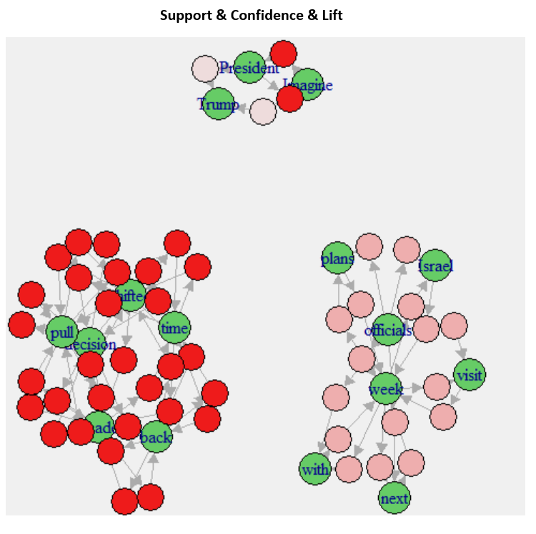
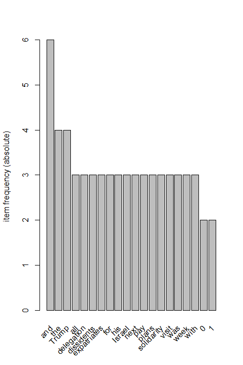
This part experimented with some other plotting methods for ARM tasks, which provides different looks to the ARM rules and linkage between nodes.
Section C: Network3D in R
Networks are mathematical graphs with nodes and edges. Network graphs can be directional, and edges can be weighted as well. In the plot above, a generic static graph/network has already experimented with. This section is looking to practice the use of Network3D and generate HTML interactive graphs. The code below in R achieves that:
networkD3::saveNetwork(D3_network_Tweets,
                       "rule1.html", selfcontained = TRUE)

)
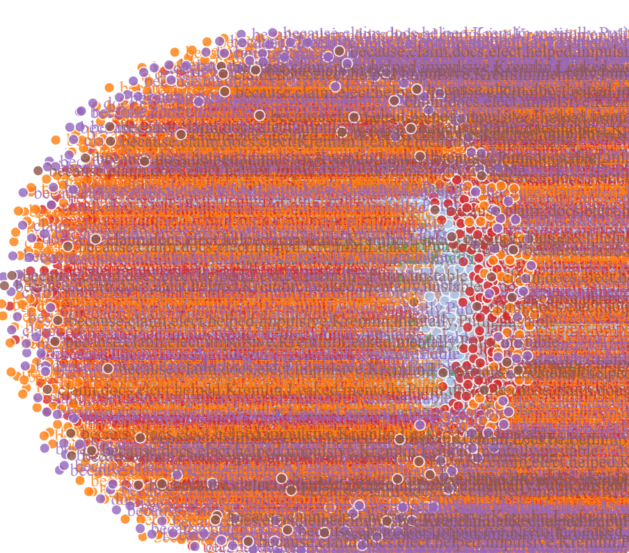
Because there are quite a number of rules generated from the apriori function(using support as 0.06), the inter-node relationship isn't very clear or too concatenated together for any insights to be discovered. So the above network graph is showing as a figure to reduce the load on the server and prevent the website from freezing. Therefore, the apriori function's parameters are adjusted to sup at 0.11(shown above) to reduce the overall output size.
 arules::apriori(transac_data, parameter = list(support=.11,
                                                  confidence=1, minlen=2))
After applying the change, the number of output rules is reduced to a great extent. Another network3d Html graph is generated.
Section D: Maps Using leaflet
This section uses the R package leaflet as the main driver for building maps showing geo data. The map data are primarily collected from the internet and is shown in the Dataset section about what is included in that dataset. The key to building maps is to have the zipped files of us, especially the county map, downloaded from the census website.
The code below loades the map files into the Rstudio environment with file explorer showing whats included in the file pack.
us.map = readOGR(dsn = ".", layer = "cb_2018_us_county_20m", stringsAsFactors = FALSE)
head(us.map)
#set back to file directory

The complete code is included in the Methodology section for reference. Below are three distinctive maps built from the leaflet. From the top, the bottom are County Female Percentage, County Water Drought Area, and County Land Area
The three maps are built using different colormap to show distinctiveness from each other. For example, while clicking on each county region on the map, it interactively shows the corresponding county name, female percentage number, water-drought area number, and land area number.
Discussion
Association Rule Mining (ARM) is a great way to find inter-relationship between itemsets in a dataset. Through this study, it is vital first to prepare a transaction dataset before analysis tasks. There are three essential rules data scientists should understand: support, confidence, and lift. The notable difference can also be found at the apriori function, where the parameters' adjustment can yield a significant difference in outcomes. The number of output is different, and how itemset on Left Hand Side(LHS) and Right Hand Side(RHD) are allocated is differed.
There are many ways to visualize the output from the apriori function. The simplest way is the print or inspects from the console in Rstudio. One can also use a scatter plot to visualize the distribution using different colormap to differentiate. Parallel graphs, interactive graphs are also useful in terms of expanding ways to look at the output.
The network 3d graph provides a more elevated and enhanced diagram, including edges and nodes linking together, and offers interactive features. You can understand the relationship between each set a lot better by dragging and dropping nodes. For example, the group "Israel, next plans visit, with" is very prominent in the tweet collected because Trump's policy is primarily associated with those words. And even after the end of his presidency, people still discuss the above words using the Trump hashtag.
The mapping function provided by the leaflet package in R is one of the most popular open-source JavaScript libraries for interactive maps. It’s used by websites ranging from The New York Times and The Washington Post to GitHub and Flickr, as well as GIS specialists like OpenStreetMap, Mapbox, and CartoDB. The more developer uses it, and other powerful tools, the better the analysis can be and the more findings can be extracted..