Methodology
Clusters, in general, represent data points that are close to each other. Data points that differ from each should reside in different clusters. Clustering is an unsupervised machine learning task that automatically divides the data into clusters or groups of similar. This section aims to use both python and R to explore clustering on two datasets collected from a previous study.
Dataset
| Dataset | Type | Description | |
|---|---|---|---|
| Data4: Acute Liver Failure | Record/Numeric Data | Contains two labels, first label Obesity indicates the person is obese or not(1 or 0), second label Obesity Level 0-5 suggests the level of obesity from underweight, normal, heavyweight, obesity class 1, obese class 2 and obesity class 3 | |
| Data6_1: Subreddit "Keto" | Corpus/Text Data | A total of 33 text files in the corpus. Each text file is a submission from a Reddit user about his/her keto diet experience. Generated previously during the data cleaning process |
Section A Clustering with Python
This section only uses python for clustering and visualizing clusters etc. Kmeans clustering is applied to both record data and corpus data. Hierarchical clustering with dendrogram created for record data and word cloud created for corpus data. Also created three distinct distance metrics with heatmap: Euclidean Distance, Manhattan Distance, and Cosine Distance for both record data and corpus data
A - 1: Record Data
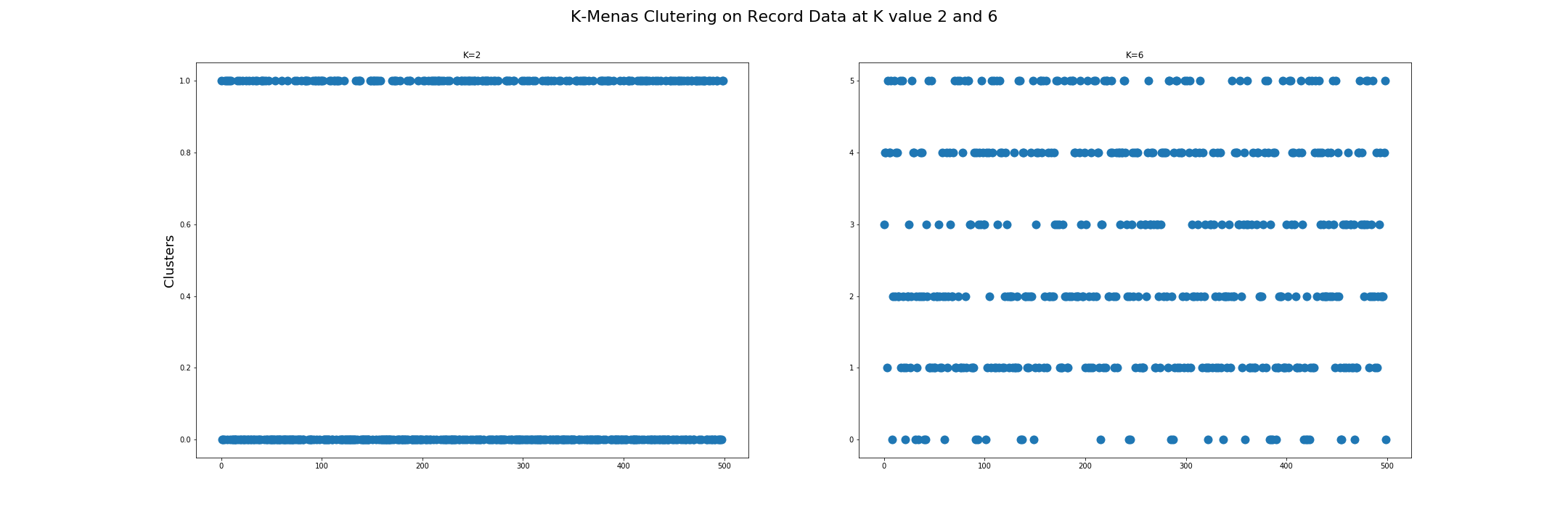
The first visualization shows K-Means Clustering on Record Data at K values 2 and 6. As explained in Datasets above, record data has two labels, one with two outcomes and one with six outcomes. They were both removed before the clustering process.


The above two visualization shows K-means Clustering on Record Data at K values 2 and 6 using 3D plots. Each visualization is a comparison between existing labels and KMeans Model prediction. The color difference is present, and the extent of which is evident.
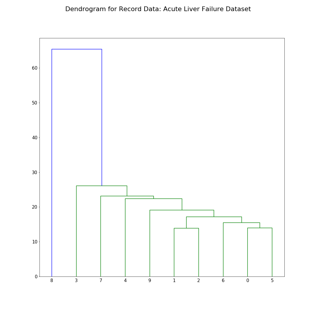
In this visualization, only ten rows are selected from the record dataset to demonstrate hierarchical clustering. The dendrogram provides a clear linkage between rows that are close to each other. The distance metric used here is Euclidean Distance.
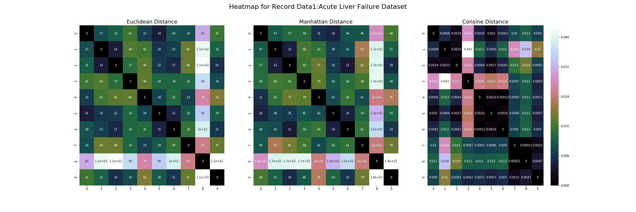
The three visualizations above show three different distance metrics for record data. The data1 in the title is how I addressed the record data in the script. On the left is the Euclidean Distance, the center is Manhattan Distance, on the right is Cosine Distance.
A - 2: Corpus Data

The visualization above shows K-Means Clustering on Corpus Data at K values 2, 3, and 4. The x-axis is the file names from the corpus. The y-axis is the clusters at the integer level.
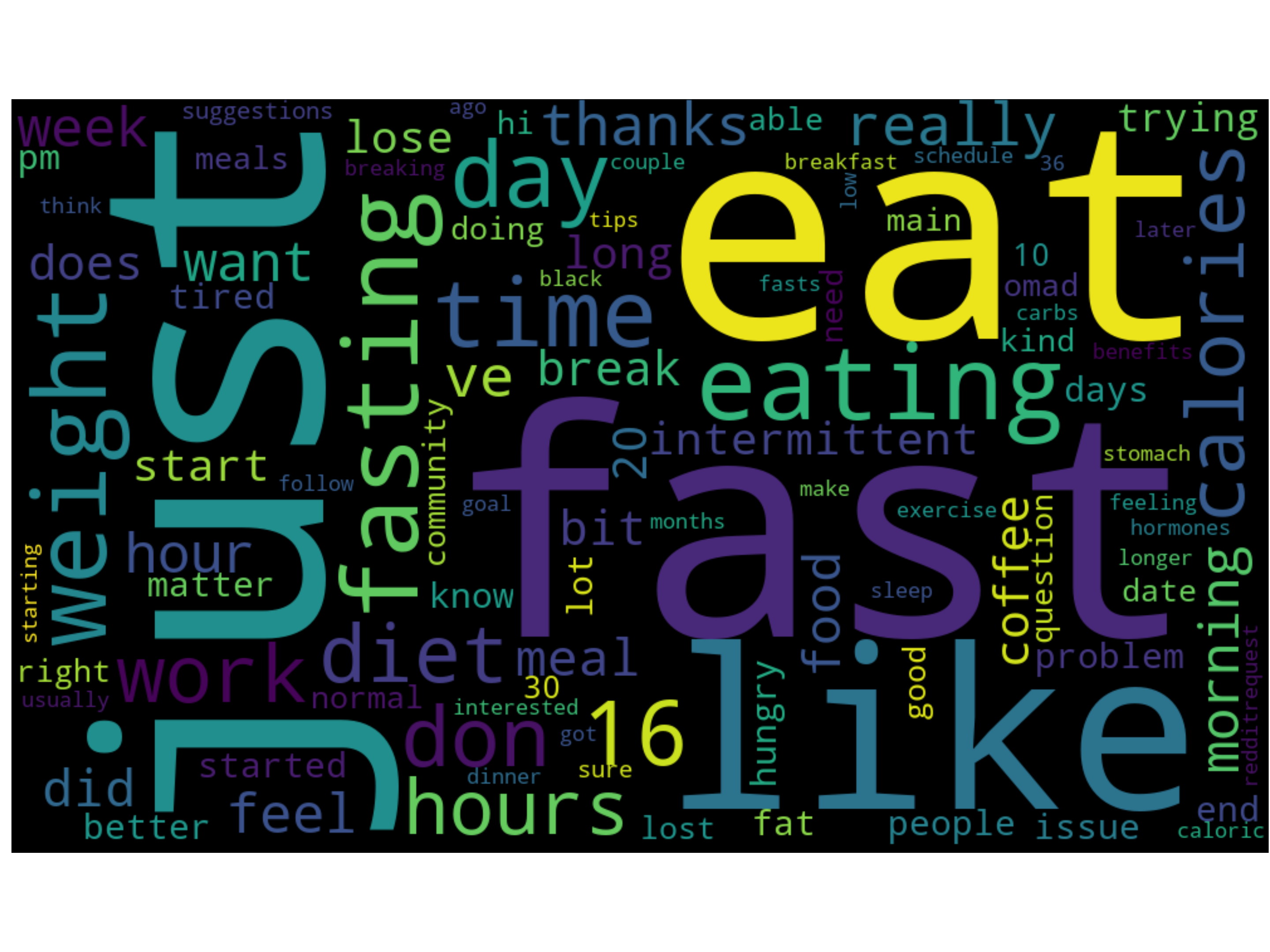
The word cloud generated with words and frequencies with CountVectorizer. Stopwords and common words are removed from the list. Since the corpus data is about ketogenetic diet submission on Reddit, most words circulate the topic of food and diet.
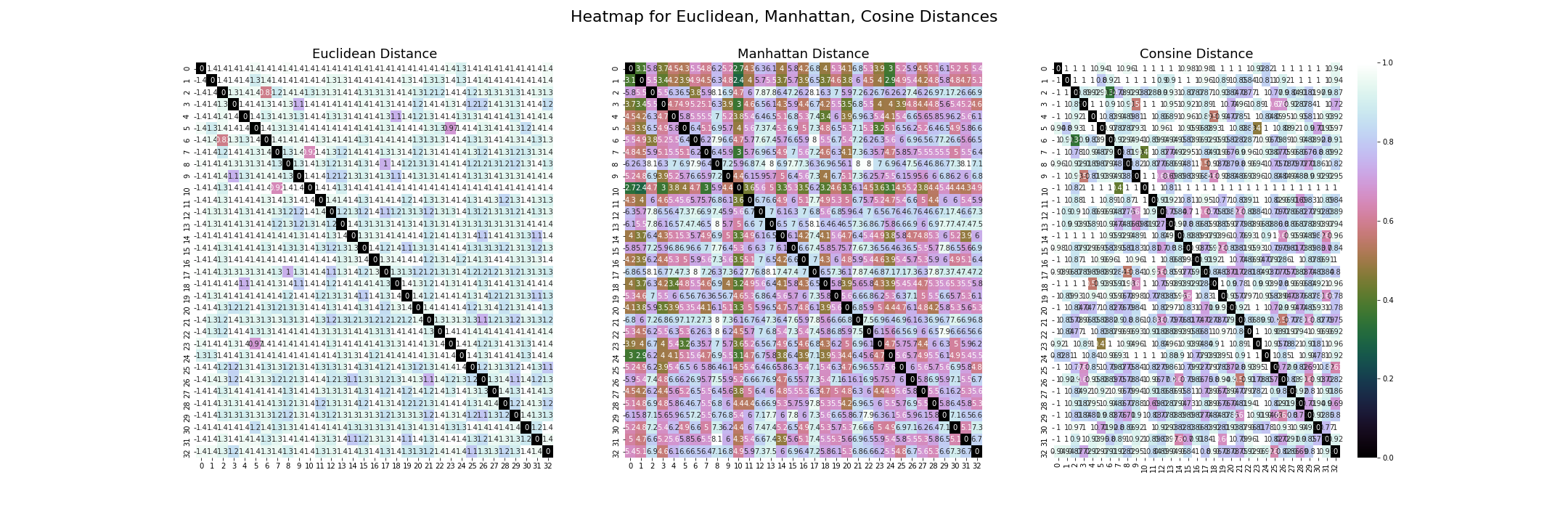
The heatmaps here are using the same method as the one above. Three distinct distance metrics are shown. Both axes show the name of the corpus text file.
Section B: Clustering with R
This section only uses R for clustering and visualizing clusters etc. Kmeans clustering was applied to record data and corpus data and visualized using fviz_cluster. Hierarchical clustering with dendrogram created for both record data corpus data. For record data, Euclidean Distance, Manhattan Distance, and Cosine Distance are used to generate hclust dendrogram. For corpus data, Euclidean Distance, Manhattan Distance, and Minkowski Distance are used to create hclust dendrogram for both TermDocumentMatrix and DocumentTermMatrix. DBSCAN, elbow, Silhouette, and Gap Stat functions applied to both data.
B - 1: Record Data
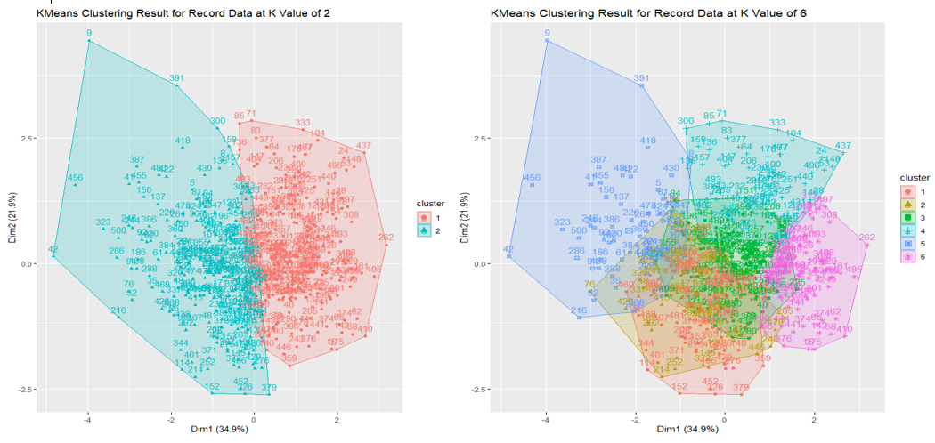
Because record data has two label columns, as shown in the table above, two KMeans clustering is applied at k values 2 and 6.
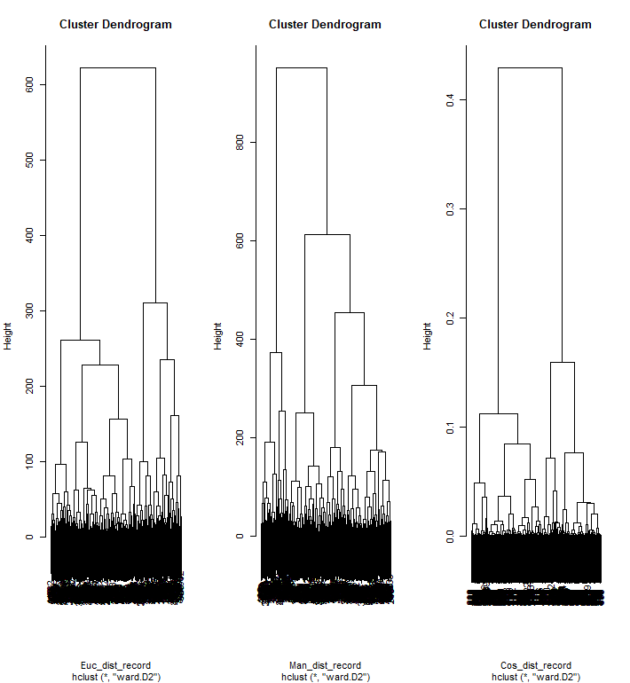
For the dendrogram, three different distance metrics are used to show the difference between each distance metric. The bottom linkages are densely combined due to the record data's size, not an ideal way to visualize.
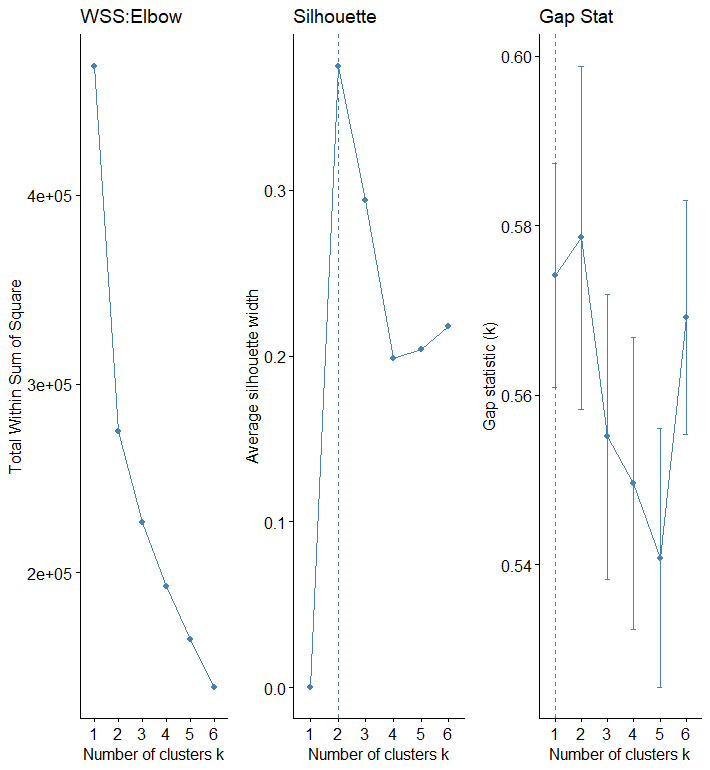
As required, using elbow, silhouette, and gap stat methods checks for the optimal number of clusters to use in KMeans clustering. For the record data, all methods show that two should be the optimal number for k.
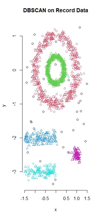
The dbscan method is density-based clustering for arbitrary shapes. It does a good job here to identify different regions and give them defining shapes.p>
B - 2: Corpus Data
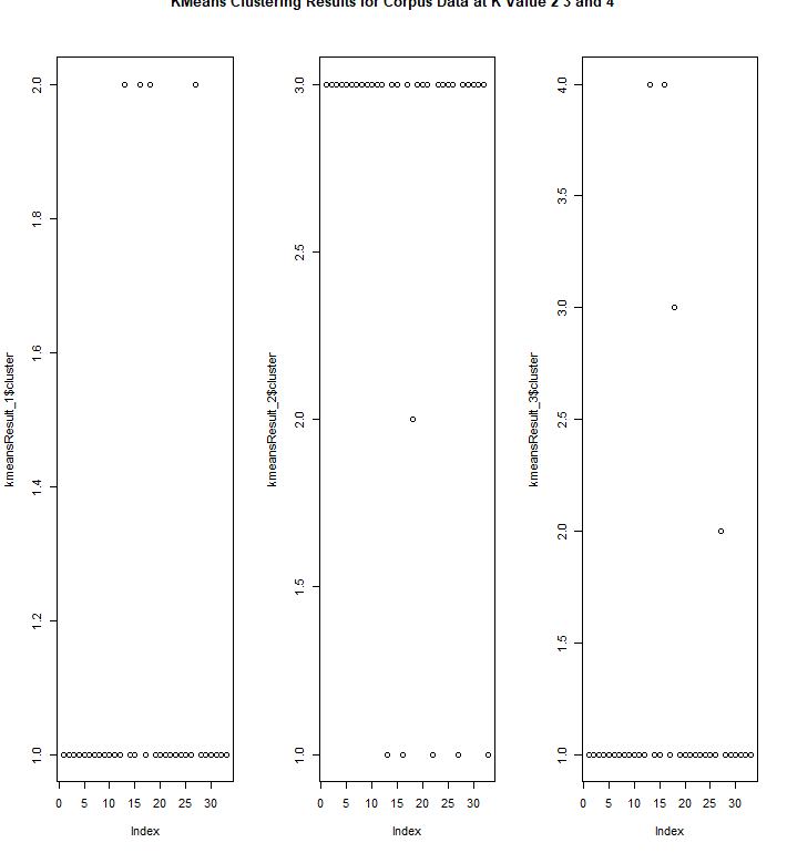
For KMeans clustering on corpus data, fviz_cluster wasn't used because a regular plot should pick up where each cluster is located.
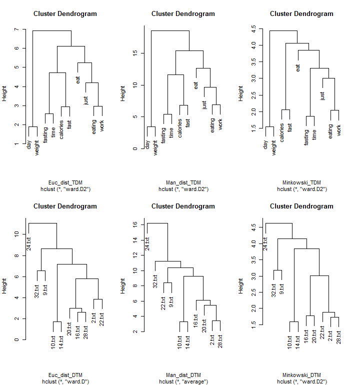
The dendrograms are created with hclust function with Euclidean, Manhattan and Minkowski Distance. When reading into the corpus, bothTermDocumentMatrix(TDM) and DocumentTermMatrix (DTM) are created. The top 3 figures are for TDM and the bottom 3 figure are for DTM.
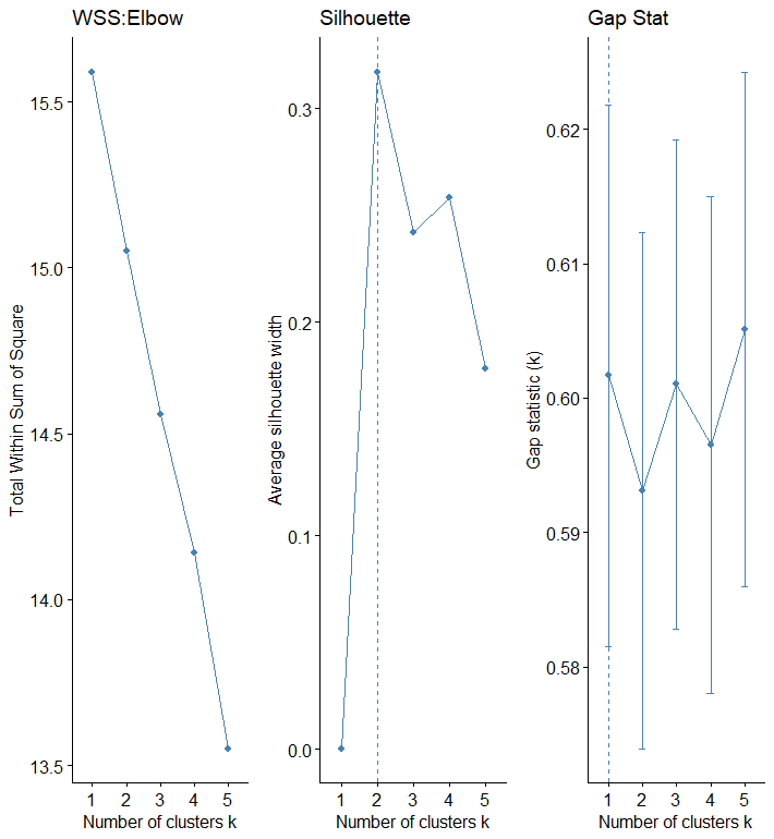
The elbow, silhouette, and gap stat methods are applied to the corpus data as well. Looking at each approach, the optimal number for K is not as straightforward as recorded data. In the elbow, the optimal number looks like to be 2 or 3, while in Gap stat, the optimal number seems to be 5.
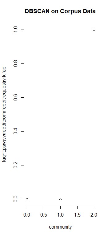
Density-based clustering for corpus data here, however, it does not seem to be better fitted than the previous two clustering method.
Discussion
Clustering is an unsupervised machine learning method that automatically divides data into groups. Different clustering methods like K-Means Clustering, Hierarchical Clustering, and Density-based Clustering (DBScan)provides unique capabilities and strengths. The use case for each clustering method depends on the distribution of the data points and type. For K-Means clustering, it is essential to conduct preliminary research on selecting the optimal number for K, as it dictates how many clusters are created. Elbow, Silhouette, and Gap-Stat are explored in this study. It is most wise to use all three or two of the three methods simultaneously to find the optimal number for K, use one for a more naive elementary approach, and use the other for validation.
In K-Means Clustering, the Euclidean distance is mostly used. This study explored three other distance metrics: Manhattan Distance, Cosine Distance, and Minkowski distance. Minkowski Distance is the generalized form of Euclidean Distance, depending on the parameter p, which one can specify a number to. It can also represent Euclidean Distance and Manhattan Distance. In R, this has been used for generating dendrogram. Manhattan Distance is usually preferred over the Euclidean Distance metric. The data dimension increases due to the notion curse of dimensionaility. The Cosine Distance or Cosine Similarity is mainly used to find similarities between two data points. When the cosine distance increases, the cosine similarities decreases.
The convergence is guaranteed for K-Means Clustering. For Hierarchical Clustering, the number of clusters is not required before the clustering process. One can stop at any number of clusters and find appropriate numbers by interpreting the dendrogram. The dendrogram in hierarchical clusters provides lots of flexibility and ease of handling of any forms of similarity or distance metrics. When displayed through heatmap with a colormap, distance metrics help identify rows or features close to each other. The third popular clustering method is DBSCAN, or density-based clustering. The main advantage of using DBScan is to detect outliers and handling noise presented in the dataset as clusters are formed as arbitrary shapes. Contrary to K-Means clustering, which uses the similarity between data with Euclidean distance, DBScan does not require K's specification and uses radius and minimum points to separate high densely populated areas from the low-density region. However, it is not as efficient for a high-dimensional dataset as the K-Means clustering method.