Methodology
Naive Bayes or NB a family or collection of algorithms that assume that the features being classified are independent of all other features. Naïve Bayes classifiers are highly scalable, requiring a number of parameters linear in the number of variables (features/predictors) in a learning problem. Maximum-likelihood training can be done by evaluating a closed-form expression, which takes linear time rather than by expensive iterative approximation used for many other classifiers.
There are some attributes that is unique to Naive Bayes: in summary
Support Vector Machines or SVM is a supervised machine learning technique. It uses known and labeled data to “train.” It uses different “kernel” options such as linear, gamma, sigmoid, and Gaussian. SVM can perform feature transformation into higher dimensional space (or infinite Hilbert Space) so that input vectors (x) are separable by some hyperplane (high dimensional plane). If you need data separated into more than two groups, you will need more than one SVM. Each SVM classifies as Class 1 or Class 2. Most “important” training points are called support vectors; they define the hyperplane.
In this study, both python and R will be used to explore the above two concepts in two different sections. Each section will talk about python first, then R. The corpus Data has two sets in it, representing two subreddit submissions from "Keto" and "intermittent fasting." The record data is a revisit, an already cleaned version of Data4:Acute Liver Failure data. The detail of which layed out below.
Dataset
| Dataset | Type | Description | Condition |
|---|---|---|---|
| Data6_1: Subreddit "Keto" | Corpus/Text Data | Derived from corpus generated from previous study, this dataset only consists of indexing number and content of each subreddit submission. | To convert into transaction data, it requires the removal of punctuations, special characters, etc |
| Data6_2: Subreddit "intermittentFasting" | Corpus/Text Data | Derived from the corpus generated from the previous study, it consists of 33 text files and one compressed file. Each text file is a Reddit submission from the user. | Perform decision tree on corpus data requires tokenization activities and generate new dataframe |
| Data4: AcuteLiverFailure(modified) | Record/Numeric Data | Modified Data4, removed multiple unused columns and rows to reduce size. | Cleaned, removed additional label |
Section A: Naive Bayes
This section explores Naive Bayes in both python and R on record data and corpus data. Presentation for each small section will go over python first, then shift to R. To implement Naive Bayes in python. from sklearn.naive_bayes import MultinomialNB
, in R, library(naivebayes) will be heavily used. Those packages are making building Naive Bayes models easy. Additionally, is the use of confusion matrix will be included for each model creation. It is also offered by sklearn..
A - 1: NB on Record Data
For the record data, read in the record.csv file using pandas, then split the training set and testing at 30%. Record the label from both test and train set, then drop the label column before fitting into the model. The code below should demonstrate the process:
recordDF = pd.read_csv("path")

#generate train and test set
TrainrecordDF, TestrecordDF = train_test_split(recordDF, test_size=0.3)

###save and remove label from train and test
TrainrecordLabels=TrainrecordDF["Obesity Level 0-5"]
TestrecordLabels=TestrecordDF["Obesity Level 0-5"]
print(TestrecordLabels)

#remove labels
TestrecordDF= TestrecordDF.drop(["Obesity Level 0-5"], axis=1)
print(TestrecordDF)

TrainrecordDF = TrainrecordDF.drop(["Obesity Level 0-5"], axis=1)
print(TrainrecordLabels)
Now first thing is to initiate the Naive Nayes in python. Then fit the training variables and training label variable to the Naive Bayes model previously declared. Use predict on the test set to generate a list of predictions. To compare the accuracy of the Naive Bayes algorithm, using a confusion matrix is straightforward and efficient. The code below demonstrates the process.
MyModelNB= MultinomialNB()

NBrecord=MyModelNB.fit(TrainrecordDF, TrainrecordLabels)
Prediction1 = MyModelNB.predict(TestrecordDF)
# Confusion Matrix
record_NB_cf = confusion_matrix(TestrecordLabels, Prediction1)

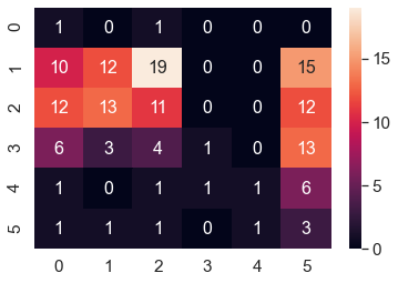
There are a total of 6 labels. Each label represents a level of obesity. From the graph, the left axis indicates the true label; the bottom axis indicates the predicted class. Lots of points are distributed among obesity levels 1 -3. This distribution suggests the majority of the population in the dataset is like to be 1-3 with very few people at level 5(overweight) 0 (underweight)
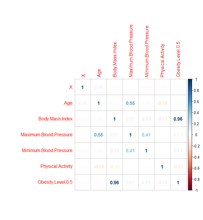
In R, before exploring Naive Bayes. The code here: correlationMatrix = cor(temp, use="complete.obs")
helps explore the relationship between columns and what might be a strong variable for predicting labels. The plot below shows this relationship:

The body mass index column has the most effect on Obesity level at 0.96. This is because that is how categorization on obesity level was done initially.
A similar approach was then applied by reading in the CSV file, factor the label column, generate the training and testing set, and then build the Naive Bayes Classifier. Keep in mind, here labels from both the train and test set are removed. Then, predictions were made to compare with the true label from the test. To generate the confusion matrix, use the table function to do that, and here is the code to demonstrate the process:
recordDF$Obesity.Level.0.5 = as.factor(recordDF$Obesity.Level.0.5)
NB_DF_Train = subset(NB_DF_Train, select = -c(Obesity.Level.0.5))
NB_DF_Test = subset(NB_DF_Test, select = -c(Obesity.Level.0.5))
(NB = naiveBayes(NB_DF_Train, NB_DF_TrainLABELS, laplace = 1))
table(NB_Pred,NB_DF_TestLABELS)

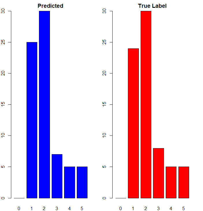
Quite different from what gathered in python, the majority of the predictions are made correctly. This might incite further investigation in the future. For now, Naive Bayes indicates a practical tool for supervised learning on record data.
A-2: NB on Text Data
For text data, there are two corpus sets. Each one contains about 30 subreddit submissions. Python will be discussed first, then R. Tokenization in python is done in 4 ways, countvecrizer with Stemmer, CountVectorizer with Bernoulli, TfidVectorizer, and TfidVectorizer with Stemmer. The specifications of each vectorization method will be skipped here and also in section B below. Each tokenized data frame will be fitted into a Naive Bayes model and generate a total of four confusion matrix plot.
STEMMER=PorterStemmer()
print(STEMMER.stem("fishings"))

# Use NLTK's PorterStemmer in a function
def MY_STEMMER(str_input):
    words = re.sub(r"[^A-Za-z\-]", " ", str_input).lower().split()
    words = [STEMMER.stem(word) for word in words]
    return words

MyVect_STEM=CountVectorizer()
MyVect_STEM_Bern=CountVectorizer()
MyVect_IFIDF=TfidfVectorizer()
MyVect_IFIDF_STEM=TfidfVectorizer()
Looking at each confusion matrix from an accuracy standpoint, the TfidVectorizer got most of the predictions correct. This might be an indication of more applicable uses in future language processing tasks.
For tokenization in R, , document term matrix(DTM) was used and here generated a data frame based on the DTM. The first step is to clean up the corpus, then adding labels to the end of the document term matrix column. Finally is to apply a similar approach to analysis on record data. The result of which is shown below:
Frankly speaking, the accuracy is not ideal, maybe due to how data was set up and converted to a data frame initially. This study's two corpora have many overlapping topics and interest points, as they are all about health, fitness, and obesity-related. The subreddit "Keto: is very intertwined in the intermittent fasting community, so, understandably, misprediction occurs. For future data, the corpus set should be picked in distinct fields where the majority difference is very much needed and should be evident from the start.
Section B: Support Vector Machines
Support Vector Machines or SVM in python and R have similar approaches and implementations. In python and R, the kernel type can be adjusted between linear, polynomial, and radial basis functions. The cost level of each type of kernel is also something one can experiment with. Initialization of each model was done first, then fit the training data on the model with predictions generated. The confusion matrix will still be the clear indicator of the accuracy of the prediction and model performance. The preprocessing method of each data will be skipped here.
B - 1: SVM on Record Data
The image below shows three different kernels. Here, the polynomial kernel performed the best and got most of the predictions correct. The interesting thing is that most people are at obesity level 1-3, similar to what NB find out in R earlier.
The image below shows 3 SVM different kernels in R. Keep in mind the kernel order is different. In R, the linear kernel actually performs the most accurate in terms of label prediction relative to the other two kernels.
B - 2: SVM on Text Data
Here in python, the visualization below is showing one model using only the "CountVectorizer with Bernoulli" tokenization method, then fitted it with three different kernels. The confusion matrix for each model plottd using heatmap. It seems that for this particular model scenario, the linear kernel produces a good result.
The linear SVM kernel produced acceptable results. Then the SVM linear kernal is applied to 4 different tokenized data; From the plot, CountVectorizer with Stemmer have identical outcomes when it comes to prediction results.
In R,Since the tokenization is done with the document term matrix, a single confusion matrix output is plotted, showing 1 model with three different SVM kernel. However, neither of which is particularly impressive. Same as before, this could relate to how the corpora are tokenized or cleaned. Another hypothesis could be the tokenization in python may perform better and more complete than R.
Discussion
To recap some of the critical information regarding Naive Bayes and Support Vector Machine. One thing fascinating about using python and R is the wide selection of machine learning packages and community support. This makes adjusting the parameters of a specific function and tweaking small elements in code super easy. Mathematically, both naive Bayes and support vector machines are equally strong and versatile and can be applied to different applications. Practically, there are distinctions from this study regarding prediction accuracy and generates credible outcomes. Whichever to use requires adjustment and improvement made to the model like switching to a different kernel, alter parameter values, etc. In this study's scope on obesity, it shouldn't be overlooked that the two corpus data should have more distinction in order for the model to differentiate as the results do not converge very well. The record data, which purely predicts the obesity level based on several independent variables, is quite accurate. Most people are at obesity level 1-3, which considers the size and the distribution of the data, is unbalanced and probably should either decrease the amount of level 1-3 people or add more people with a level other than 1-3. Those can be potential improvements for later projects.