Methodology
Decision Tree is one of the supervised predictive modeling approaches used in statistics, data mining, and machine learning. It uses a decision tree (as a predictive model) to go from observations about an item (represented in the branches) to conclusions about the item's target value (represented in the leaves). Tree models where the target variable can take a discrete set of values are called classification trees; in these tree structures, leaves represent class labels, and branches represent conjunctions of features that lead to those class labels. Decision trees where the target variable can take continuous values (typically real numbers) are called regression trees. Decision trees are among the most popular machine learning algorithms, given their intelligibility and simplicity.
Aside from the conceptual ideas. there are several key parameters to note:
Gini impurity is how often a randomly chosen element from the set would be incorrectly labeled if it was randomly labeled according to the distribution of labels in the subset. A GINI Value of 1 or 0 means the node is pure.
Information gain: is based on the concept of entropy and information content from information theory. It helps determine the strength of a partition by comparing the purity of the parent node (before split) to child nodes (after the split). The Gain (∆) is a measure for goodness of split.I is the impurity measure of a node, N is the number of records at the parent node, k is the number of attribute values. N(vj) is the number of records in child vj. If entropy is used as the impurity measure, the difference in entropy is the information gain. *An entropy value of 0 means the node is pure.
Confusion Matrix: is a specific table layout that allows visualization of the performance of an algorithm, typically a supervised learning one (in unsupervised learning, it is usually called a matching matrix). Each row of the matrix represents the instances in a predicted class, while each column represents the instances in an actual class (or vice versa). We will see an example of this in later visualizations.
Random Forest is a tree-based machine learning algorithm that leverages multiple decision trees' power for making decisions. As the name suggests, it is a “forest” of trees!
Dataset
| Dataset | Type | Description | Condition |
|---|---|---|---|
| Data6_1: Subreddit "Keto" | Corpus/Text Data | Derived from corpus generated from previous study, it consists of 34 text files and 1 compressed file. Each text file is a reddit submission from user. | Perform decision tree on corpus data requires tokenization activities and generate new dataframe. |
| Data6_2: Subreddit "intermittentFasting" | Corpus/Text Data | Derived from the corpus generated from the previous study, it consists of 33 text files and one compressed file. Each text file is a Reddit submission from the user. | Perform decision tree on corpus data requires tokenization activities and generate new dataframe |
| Data4: AcuteLiverFailure(modified) | Record/Number Data | Modified Data4, removed multiple unused columns and rows to reduce size. | Cleaned, removed additional label in Section A |
Section A: Prepare Data for Decision Tree
This section is dedicated to preparing a dataset for decision tree and random forest tasks in both python and R. For the python decision tree task, two corpora will be generated and one record dataset for the R tasks.
A - 1: Create Two Corpus Text Dataset
The code below demonstrates how corpus text files are generated. The files are named with numbers in order for simplicity reasons.
if not os.path.exists(txt_dir):
    os.mkdir(txt_dir)
print(data6_1_null_rmed.iloc[1,4])
#generate txt corpus for word processing, input dataframe, root directory for storing, and the column number
for i in range(data6_2_null_rmed.shape[0]):
    f = open(os.path.join(txt_dir + str(i) + '.txt'),'w', encoding='utf-8')
    f.write(data6_2_null_rmed.iloc[i,4])
    f.close()

data6_1_null_rmed.to_csv(os.path.join(txt_dir,'data6_1_na_removed.csv'))
data6_2_null_rmed.to_csv('data6_2_na_removed.csv')
Over the last several assignments, the extraction of each text file content has also complete. Below is a snapshot of what it looks like in a data frame format.

A-2: Clean Up Record Dataset
Clean up the recorded dataset is very straightforward. Since most unused columns have already been taken out in previous studies, only need to remove the extra-label column from the dataset. The figure below shows before and after removing the extra-label column.
Section B: Decision Tree and Random Forest in Python
This section only uses python for decision tree tasks. This also involves the practice confusion matrix that is plotted by heatmap and feature outputs in the console and additional exploratory study on random forests. The data used here are the two corpus dataset that will be tokenized in four different ways, as shown in the Dr.Gates tutorial file. Each tokenizer will be used to generate a data frame for decision tree activity, and one of the four will be used for random forest activity.
B - 1: Decision Tree with Confusion Matrix
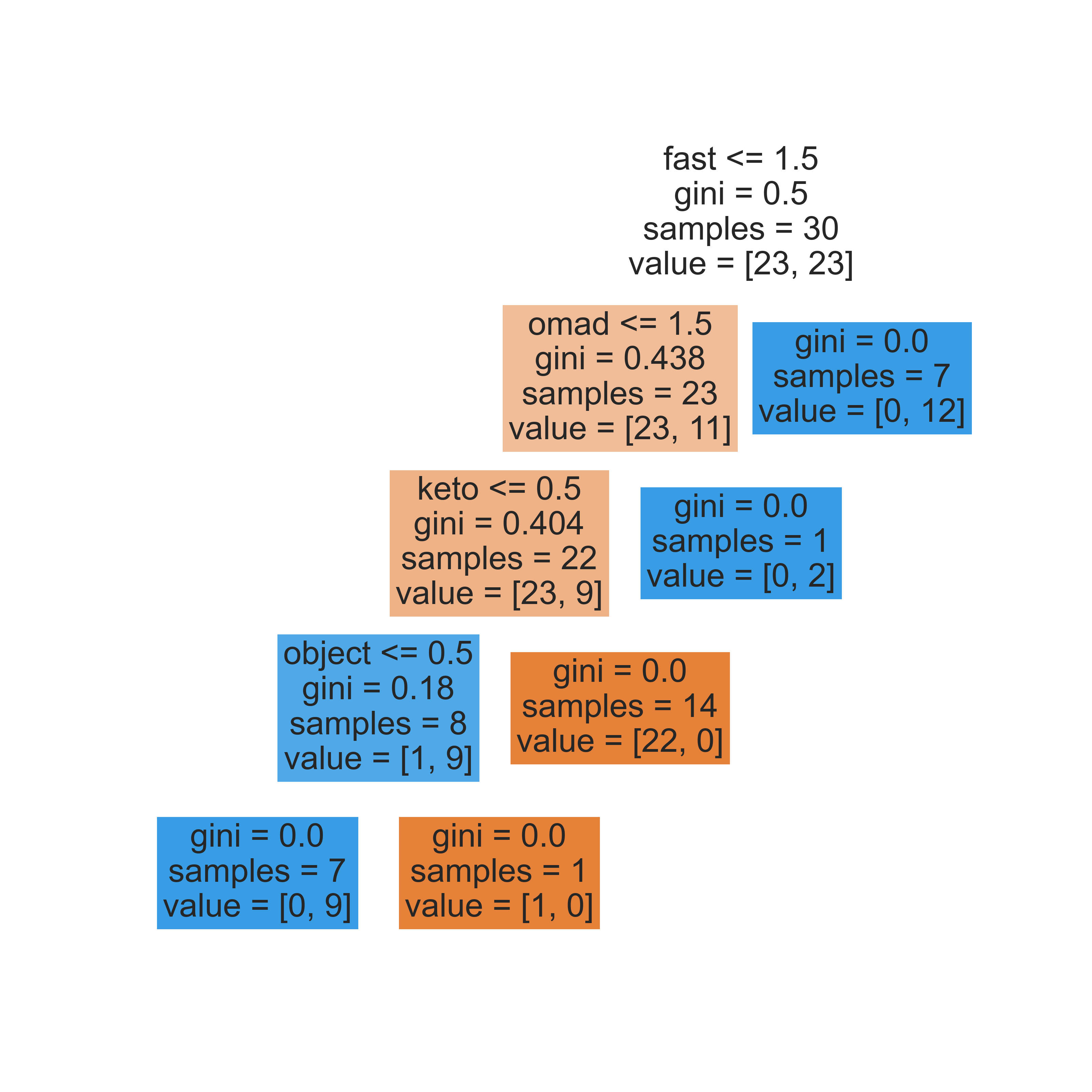
Each visualization below presents the decision tree, the confusion matrix, and the console's feature output to help explain things. The four tokenizers are CountVectorizer with Stemmer, CountVectorizer with Bernollio, TfidVectorizer, and TfidVectorizer with Stemmer. The code below demonstrates the stemmer and four tokenizer initialization.
def MY_STEMMER(str_input):
    words = re.sub(r"[^A-Za-z\-]", " ", str_input).lower().split()
    words = [STEMMER.stem(word) for word in words]
    return words
MyVect_STEM=CountVectorizer()
MyVect_STEM_Bern=CountVectorizer()
MyVect_IFIDF=TfidfVectorizer()
MyVect_IFIDF_STEM=TfidfVectorizer()
Four data frames are generated following the previous code, and each data frame is separated into a training dataset and testing dataset. Below will show the visualization of each:
The confusion matrix provides a clear indication of what is predicted correctly and what is not. The feature names are listed on the left for identification purposes. The decision tree visualization provides the critical parameters for each node, which helps understand each split's effectiveness.
B - 2: Random Forest in Python
This part explores random forest task in python with text dataset.


Section C: Decision Tree in R
The decision tree performed in R is similar in terms of logic. First, create training and test dataset from the record data, then use rpart to create various tree forms to analyze and visualize.
When using R, I learned a new trick for setting workdirectory:
# Save directory path of the current file
Directory.Path = dirname(rstudioapi::getActiveDocumentContext()$path)

# Set working directory to source file location
setwd(Directory.Path)
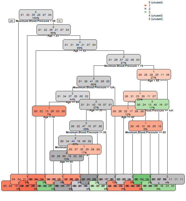
This helps set up the working directory if using a different file system like Windows, Linux, and macOS. Now back to the decision trees, below are several visualizations done for the recorded dataset. Each one further dives into more categories. As a result, some nodes are less visible.


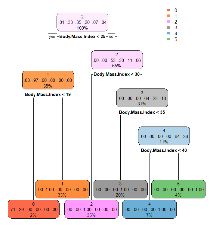
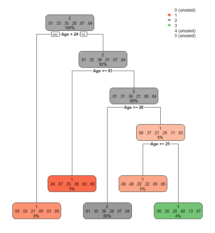
The top left visualization is done by just using the label in the rpart function. And it gives definitive and correct splits based on the BMI, which is how the data is labeled in the first place. The top right visualization is with the addition of the Age column, which seems to distribute on 1,2, and 3 only. The visualization below adds maximum blood pressure, minimum blood pressure, and physical activity column into the rpart parameter. As a result, there are a lot more splits happening. It should be pretty easy for one to identify the nodes by color, and it seems most distribution is happening on 1, 2, and 3.

Discussion
Decision Tree is a terrific supervised learning method for machine learning and deep learning tasks. It is one of the most popular ways and provides great prediction accuracy overall. From performing a decision tree and random forest tasks in python and R, a lot of attention focused on how to tokenize the text data and split training and test data as a preparation for decision tree models. For text data, the way tokenization is done can significantly impact how the model predicts and splits its nodes, as shown in Section B's visualization. Additionally, the random forests are combined with multiple decision trees for estimating purposes, which can be discussed in later studies. The confusion matrix plotted with heatmap helps reading understand what is predicted correctly and what is not.
For record data in R, things become a lot easier, as no tokenization need for record data. The rpart package and fancyRpartplot function provide direct plotting and visualizing capabilities, which is not readily available on python. It is also vital to set the correct amount of training and testing dataset from performing decision tree tasks in R. The most popular method is 7:3 or 8:2 in terms of distribution. Also, depending on the number of related columns added into the rpart function, the tree's output can look dramatically different. It is essential to select columns wisely to not overwhelm yourself with so many leaves in the output plot.
This chapter is an excellent introduction to supervised learning. A decision tree as a machine learning technique has been used in various tasks for prediction and modeling tasks.